Predict the risk of chronic kidney disease with Azure Machine Learning

In this tutorial, you will learn how to train a machine learning model in Azure Machine Learning Designer without writing a single line of code. You will create a simple classification model for chronic kidney disease prediction.

You will learn how to:

• Create an Azure Machine Learning workspace.
• Create and run a pipeline.
• Import data.
• Execute a Python script in Azure Machine Learning Designer.
• Train and evaluate a classification model.

To complete the exercise, you will need:

• An Azure subscription. If you don’t already have one, you can sign up for an Azure free account.
• The chronic_kidney_disease.csv dataset. The data has been taken from the UCI Machine Learning Repository.

Create an Azure Machine Learning workspace

You will create a Machine Learning workspace via the Azure portal.

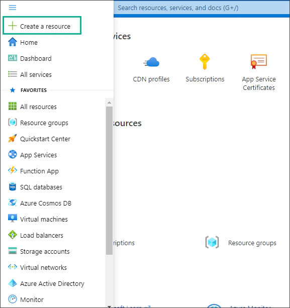
1. Sign in to Azure Portal and select Create a resource.

   

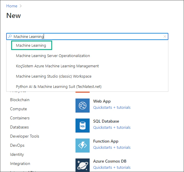
2. Search for Machine Learning and then click Create to start.

   

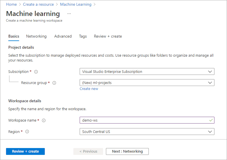
3. Configure the new Machine Learning resource. Select subscription, resource group, workspace name and region and then click Review + Create.

   

4. Wait for the workspace to be created (it may take several minutes) and then select Go to resource.

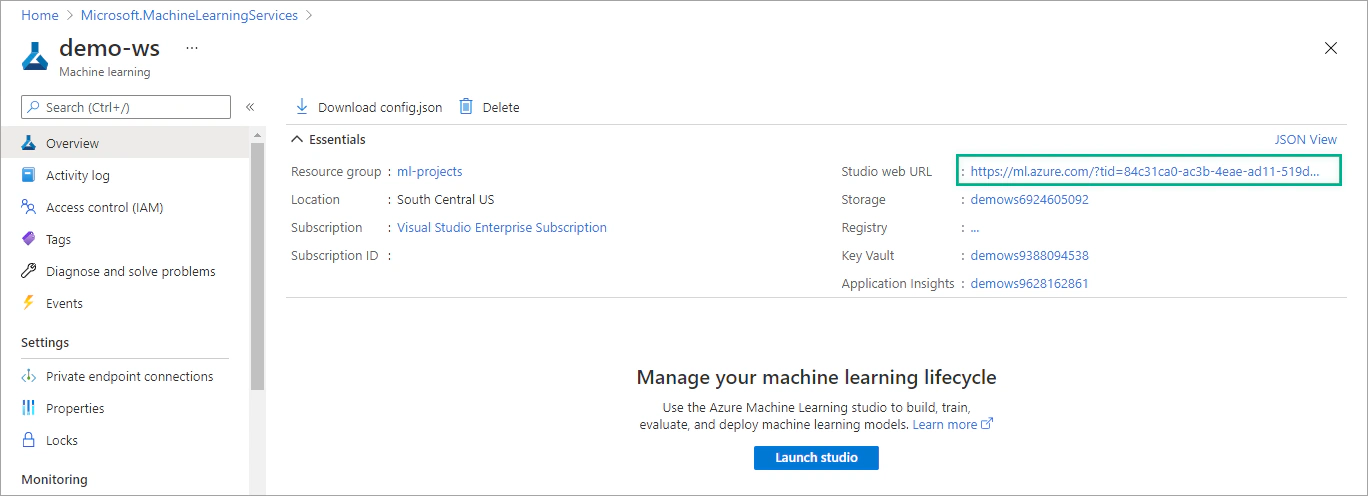
5. Click on Studio Web URL to go to your Azure Machine Learning workspace.

   

Create a dataset

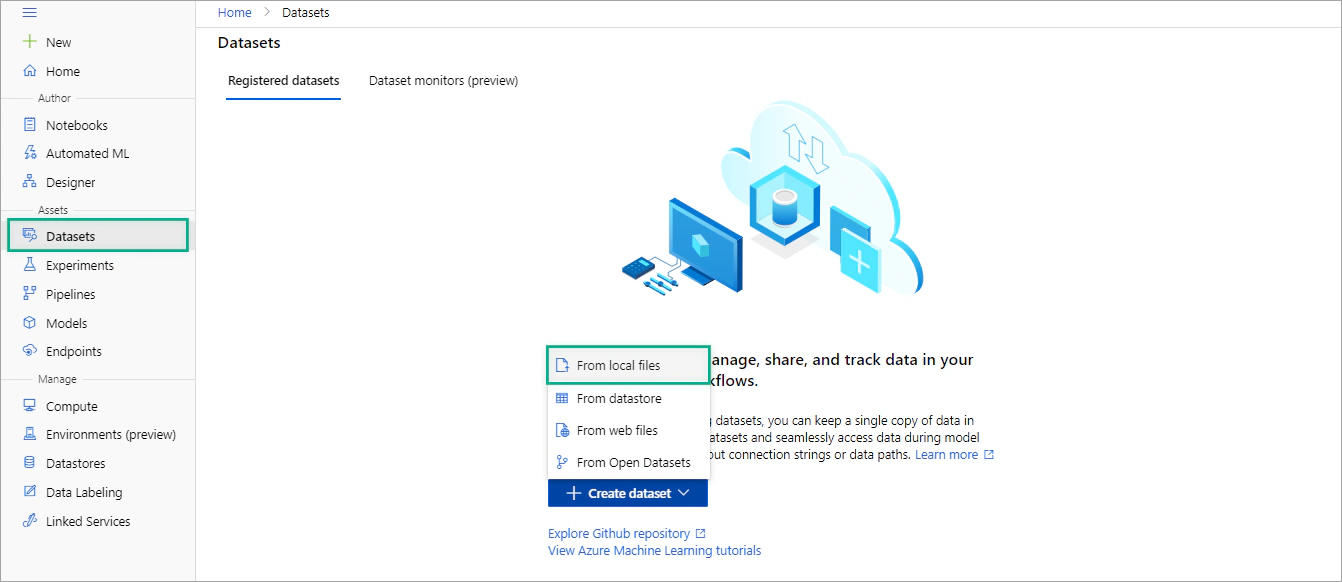
Before starting the experiment, upload the data file in your workspace.

1. In the left menu, select Datasets and then select + Create Dataset > From local files.

   

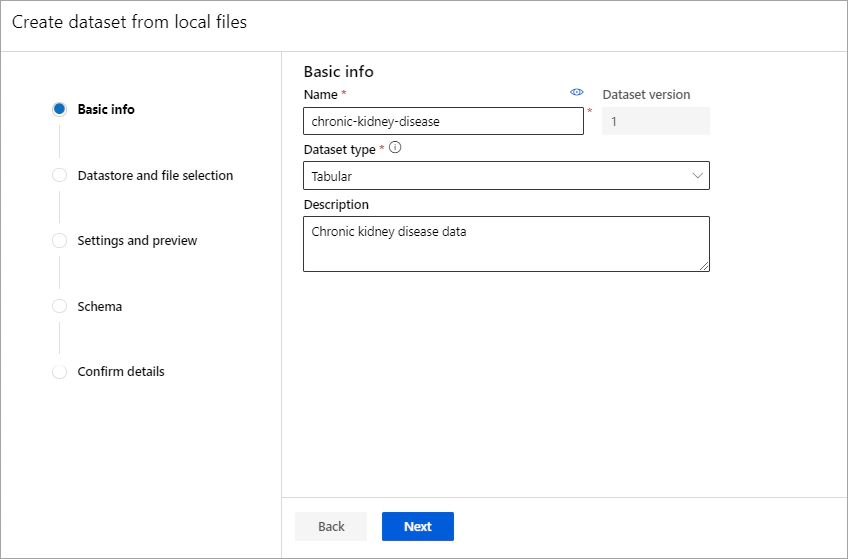
2. Provide a name and description for the dataset.

   

3. In Datastore and file selection select Browse and choose the chronic-kidney-disease.csv file on your local computer.

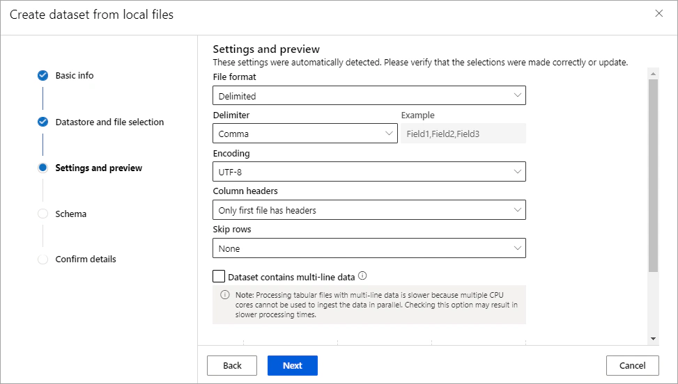
4. In Settings and preview tab, specify the following settings:

   • File format: Delimited
   • Delimiter: Comma
   • Encoding: UTF-8
   • Column headers: Only first file has headers
   • Skip rows: None
   

5. In Schema tab review the automatically detected types, select Next and then click Create.

Create a new pipeline

1. In the left pane, select Designer and then select the plus sign (+) to create a new pipeline.
2. Change the default pipeline name (Pipeline-created-on-<date>) to Prediction model for chronic kidney disease.

Set the compute target

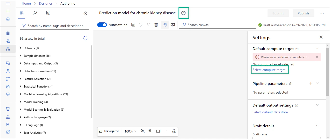
1. Next to the pipeline name, select the settings icon. In the setting pane, under Default compute target click on Select compute target.

   

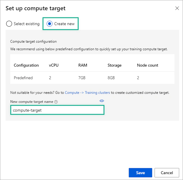
2. Select Create new, enter a name for the new compute target and then click Save. It takes several minutes for the compute target to be created.

   

Import data

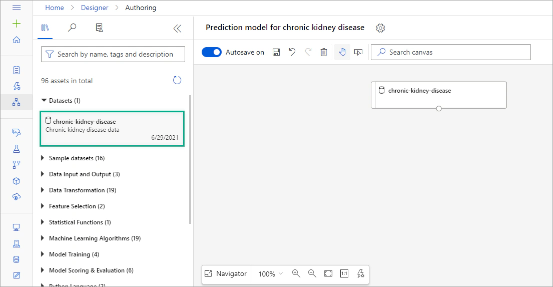
1. On the left side of the canvas, expand the Datasets section, select the dataset that you have created (chronic-kidney-disease) and drag it onto the canvas.

   

2. Right-click on the chronic-kidney-disease dataset and select Visualize. On the data visualization window, you can see statistics and histograms for each variable (column). Note that there are quite a few missing values in the dataset. We can address this issue by applying data transformations.

Add transformations

Before training the model, you will apply some transformations to the data.

1. In the left pane, expand the Python Language section and drag an Execute Python Script module to the canvas. Replace the default Python script with the following code (which converts string categories to integer values, 1 or 0):

   1 2 3 4 5 6 7 8 9 10 11 12 13

   import pandas as pd def azureml_main(dataframe1 = None, dataframe2 = None): # Map abnormal/normal to 1/0 dataframe1[['rbc','pc']] = dataframe1[['rbc','pc']].replace({'abnormal':1,'normal':0}) # Map present/notpresent to 1/0 dataframe1[['pcc','ba']] = dataframe1[['pcc','ba']].replace({'present':1,'notpresent':0}) # Map yes/no to 1/0 dataframe1[['htn','dm','cad','pe','ane']] = dataframe1[['htn','dm','cad','pe','ane']].replace({'yes':1,'no':0}) # Map good/poor to 1/0 dataframe1[['appet']] = dataframe1[['appet']].replace({'good':1,'poor':0}) # Map ckd/notckd to 1/0 dataframe1['class'] = dataframe1['class'].replace({'ckd':1,'notckd':0}) return dataframe1

2. Connect the dataset’s output port to the first input port of the Execute Python Script module.

   

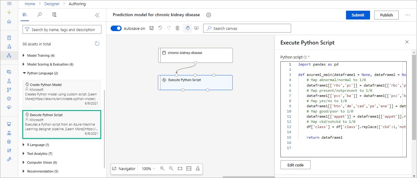
3. Add a Clean Missing Data module from the Data Transformations section and connect the first output port of the Execute Python Script module to the input port of the new module.

4. Then in its settings pane on the right, click Edit column. In the Select columns window, select With rules, in the Include dropdown list select All columns.

5. Then, set the following settings:

   • Minimum missing value ratio: 0.0
   • Maximum missing value ratio: 1.0
   • Cleaning mode: Remove entire row

6. The next step is to change the data type of the columns that you transformed using the above Python script. Drag an Edit Metadata module onto the canvas and connect the left output port of the Clean Missing Data module to the input port of the new module.

7. With the Edit Metadata module selected, in the setting pane, click Edit column. In the new window, select With rules and add the following column names in the text area: rbc, pc, pcc, ba, htn, dm, cad, pe, ane, appet, class.

8. Then, set the data type to Integer.

   

Run the pipeline

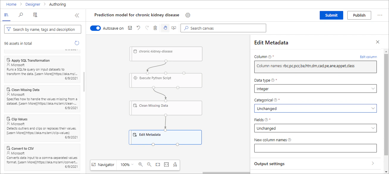
1. In the top settings menu, select Submit.

2. In the Set up pipeline run form, select Create new, enter a name for the experiment and then click Submit. Wait for the run to finish (this may take several minutes).

   

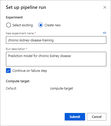
After the run completes:

1. Right click on the Edit Metadata module and select Visualize > Results dataset.

2. View the data, noting that the number of rows has been reduced and the string columns has been converted to integers.

   

Train a machine learning model

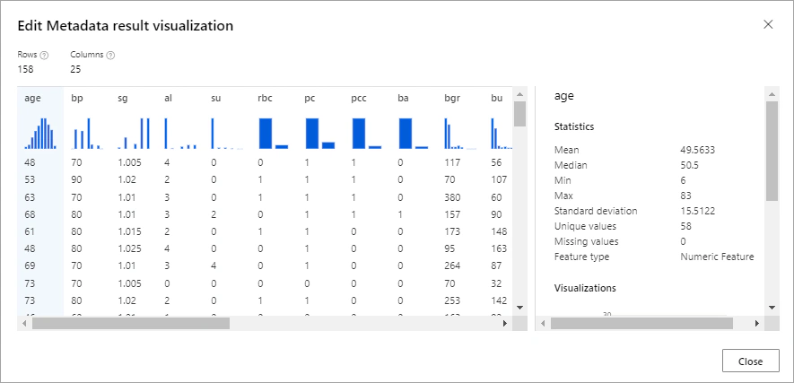
After you’ve used data transformation modules to prepare the data, you can use it to train a classification model.

Split the data

The first step is to split the data into training and test set.

1. In the left pane, in Data transformations section, drag a Split data module onto the canvas and connect the output port of the Edit Metadata module to the Split data module.

2. Select the Split data module and set the Fraction of rows in the first output dataset to 0.7. This way, you will use 70 percent of the data to train the model and 30 percent for testing the model.

   

Create a classification model

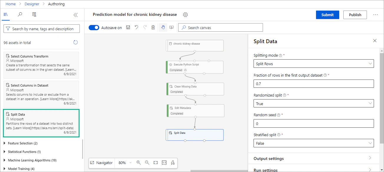
There are 2 possible classes for the label that the model will predict:

• Chronic kidney disease (1)
• Not chronic kidney disease (0)

So, we need a binary classification algorithm.

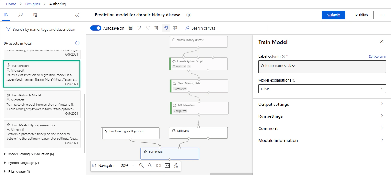
1. In the left pane, select Machine Learning Algorithms and under Classification select the Two-Class Logistic Regression module and drag it onto the canvas.

2. In Model Training section, select Train Model. Connect the output port of the Two-Class Logistic Regression module to the left input port of the Train Model module. Connect the left port (training set) of the Split Data module to the right input port of the Train Model module.

3. Select the Train Model module and in the right pane click on Edit column to select the label column (the variable that you want to predict).

   

4. The next step is to test the model. In Model Scoring and Evaluation section, select the Score Model module. Connect the output of the Train Model module to the left input of the Score Model module, and the right output (test set) of the Split Data module to the right input of the Score Model module.

Evaluate the model

In Model Scoring and Evaluation section, select the Evaluate Model module. Connect the output of the Score Model module to the left input of the Evaluate Model module.

Run the training pipeline

1. In the top settings menu, select Submit.
2. In the Set up pipeline run form, select the existing experiment and click Submit. It takes 5-10 minutes for the pipeline run to complete.

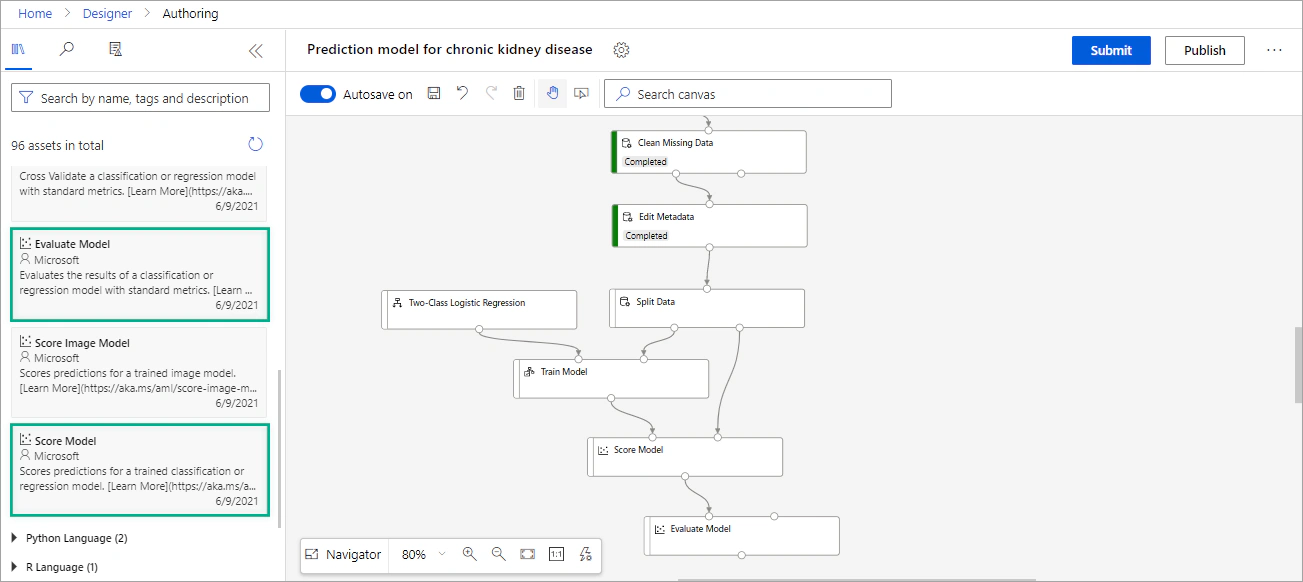
After the run completes:

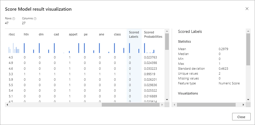
1. Right-click the Score Model and select Visualize > Scored dataset. Scroll to the right and explore the last two columns. The Scored Labels column contains the predicted label value (either 1 or 0) and the Scored Probabilities contains a probability value between 0 and 1. Probabilities greater than 0.5 result in a predicted label of 1 (chronic kidney disease), while probabilities between 0 and 0.5 result in a predicted label of 0 (not chronic kidney disease).

   

2. Then, right-click the Evaluate Model and select Visualize > Evaluation results. The result includes statistics that can help you assess the performance of the classification model. Let’s explore the confusion matrix of the model. The confusion matrix shows the predicted and actual value counts for each possible class (1 or 0).

   

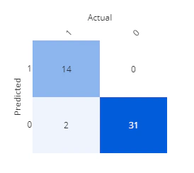
   Based on the confusion matrix:

   • There are 14 cases where the predicted and actual values are 1 (true positives).
   • There are 31 cases where predicted and actual values are 0 (true negatives).
   • In 2 cases the predicted value is 0 and the actual value is 1 (false negative)
   • There are 0 cases where the predicted value is 1 and the actual value is 0 (false positives).

You can further explore the remaining metrics or try to improve the model.

Deploy a predictive service

After creating and running the pipeline to train the model, you can create a real-time inference pipeline and publish a predictive service. If you want to publish your model, follow the instructions on my article Deploy ML model with Azure Machine Learning.

Clean-up

1. In the Azure Portal, select Resource groups on the right menu and then select the resource group that you have created.

2. Click Delete resource group.