Use IVFFlat index on Azure Cosmos DB for PostgreSQL for similarity search
Explore vector similarity search using the Inverted File with Flat Compression (IVFFlat) index of pgvector on Azure Cosmos DB for PostgreSQL.
In the previous post, you explored the IVFFlat (Inverted File with Flat Compression) index for approximate nearest neighbor search on Azure Cosmos DB for PostgreSQL. You observed that the IVFFlat index provides accurate results with lower search times compared to exact nearest neighbor search. To find out more about previous posts, check out the links below:
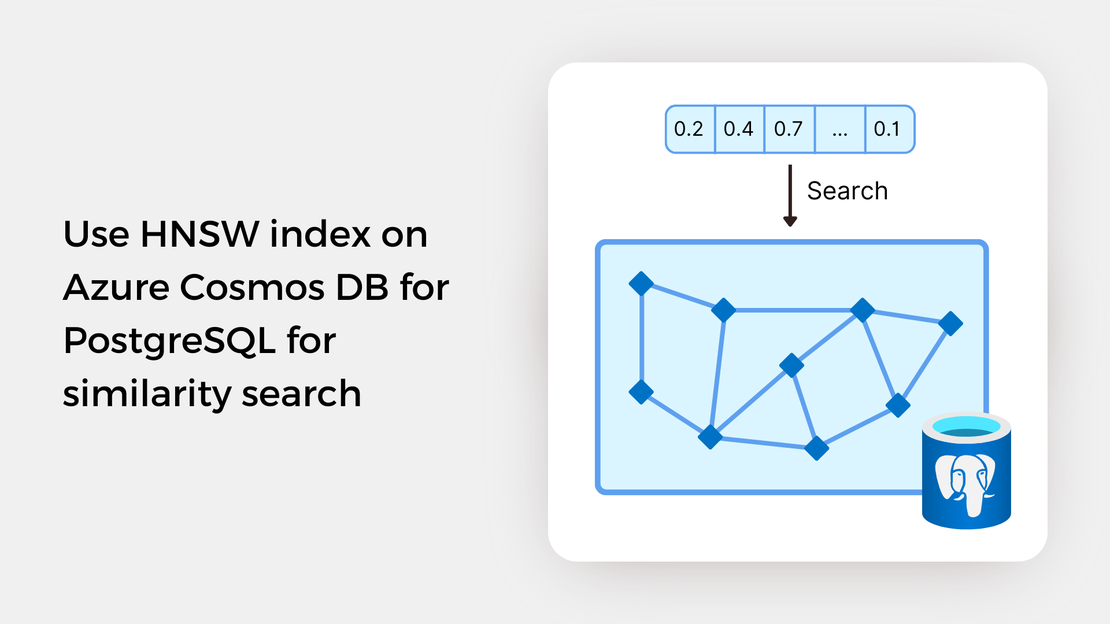
The pgvector extension provides another indexing algorithm for approximate nearest neighbor search called Hierarchical Navigable Small World (HNSW) graphs. HNSW is one of the most popular and best-performing indexes for vector similarity search. HNSW index support was introduced in pgvector 0.5.0.
In this tutorial, you will:
To proceed with this tutorial, ensure that you have the following prerequisites installed and configured:
In this guide, you’ll learn how to query embeddings stored in an Azure Cosmos DB for PostgreSQL table to search for images similar to a search term or a reference image. The entire functional project is available in my GitHub repository. If want to follow along, just fork the repository and clone it to have it locally available.
Before running the Jupyter Notebook covered in this post, you should:
Create a virtual environment and activate it.
Install the required Python packages using the following command:
| |
Create vector embeddings for a collection of images by running the scripts found in the data_processing directory.
Upload the images to your Azure Blob Storage container by executing the script found in the data_upload directory.
The HNSW index is based on the construction of a multi-layered graph structure, that is optimized for performing approximate nearest neighbor search. In this graph structure, the datapoints (also referred to as nodes or vertices) are connected to each other by edges, which make it possible to navigate through the graph by following these edges.
The base layer of the multi-layer graph essentially represents the entire dataset, while the higher layers consist of fewer nodes, providing a simplified overview of the layers below. The higher layers contain longer links, allowing for longer jumps between nodes for faster search, while the lower layers contain shorter links, enabling more accurate search. Nearest neighbor search begins at the top layer, where the longest links are present. We then navigate to the nearest node and gradually move to lower layers until a local minimum is found. This process is illustrated in the following image:
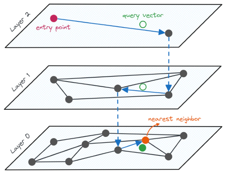
The search process in an HNSW graph can be compared to the process of planning a trip between two cities. Much like how we start our journey with major roads and gradually transition to smaller ones as we approach our destination, the HNSW search process begins with longer links at the top layer and gradually moves to lower layers as we approach the desired data points.
The HNSW algorithm is based on two fundamentals techniques: the probability skip list and the navigable small world (NSW) graphs. A detailed explanation of the process of constructing an index and searching through the graph is beyond the scope of this article. For further information, refer to the resources provided at the end of this article.
Compared to the IVFFlat index, the HNSW index generally provides better query performance in terms of the tradeoff between recall and speed, but at the expense of higher build time and more memory usage. Additionally, it doesn’t require a training step to build the index. This means you can create an HNSW index even before any data is inserted into the table, unlike the IVFFlat index, which needs to be rebuilt when data changes to accurately represent new cluster centroids.
To create an HNSW index through the pgvector extension, three parameters need to be specified:
vector_l2_ops, vector_ip_ops, and vector_cosine_ops, respectively. It is essential to select the same distance metric for both the creation and querying of the index.m specifies the maximum number of connections with neighboring datapoints per point per layer. Its default value is 16.ef_construction defines the size of list that holds the nearest neighbor candidates when building the index. The default value is 64.To create an HNSW index in a PostgreSQL table, you can use the following statement:
| |
To search for similar images through the HNSW index of the pgvector extension, we can use SQL SELECT statements and the built-in distance operators. The structure of a SELECT statement was explained in the Exact Nearest Neighbor Search blog post. For approximate nearest neighbor search, an additional parameter needs to be considered to use the HNSW index.
The ef_search parameter specifies the size of the list that holds the nearest neighbor candidates during query execution. The default value is set to 40. The ef_search parameter can be altered (for a single query or a session) using the following command:
| |
To check whether PostgreSQL utilizes the index in a query, you can prefix the SELECT statement with the EXPLAIN ANALYZE keywords. An example of a query plan that utilizes the HNSW index is provided below:
| |
Additionally, it is important to note that pgvector only supports ascending-order index scans. This means that the following query does not utilize the HNSW index:
| |
One possible way to rewrite the SELECT statement to use the index is provided below:
| |
In the Jupyter Notebook provided on my GitHub repository, you’ll explore text-to-image and image-to-image search scenarios. You will use the same text prompts and reference images as in the Exact Nearest Neighbors search example, allowing for a comparison of the accuracy of the results.

Feel free to experiment with the notebook and modify the code to gain hands-on experience with the pgvector extension!
The pgvector extension and PostgreSQL provide additional features that you can leverage to build AI-powered search applications. For example, you can integrate vector search with conventional keyword-based search methods into hybrid search systems, which generally have better performance.
If you want to learn more about the HNSW algorithm, check out these learning resources:

Explore vector similarity search using the Inverted File with Flat Compression (IVFFlat) index of pgvector on Azure Cosmos DB for PostgreSQL.
Learn how to write SQL queries to search for and identify images that are semantically similar to a reference image or text prompt using pgvector.

My presentation about vector search with Azure AI Vision and Azure Cosmos DB for PostgreSQL at the Azure Cosmos DB Usergroup.

My presentation about vector search with Azure AI Vision and Azure Cosmos DB for PostgreSQL at the virtual show MVP TechBytes.