Use HNSW index on Azure Cosmos DB for PostgreSQL for similarity search
Explore vector similarity search using the Hierarchical Navigable Small World (HNSW) index of pgvector on Azure Cosmos DB for PostgreSQL.
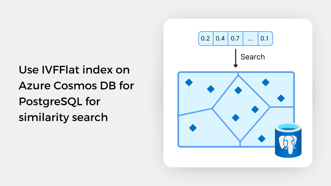
In the previous post, you developed an image similarity search app using Jupyter Notebook. Utilizing the pgvector extension on Azure Cosmos DB for PostgreSQL, you were able to detect images that are semantically similar to a reference image or a text prompt. To find out more about previous posts, check out the links below:
By default, pgvector performs exact nearest neighbor search, calculating the similarity between the query vector and every vector in the database. While this type of search provides perfect recall, it often leads to longer search times. To enhance efficiency for large datasets, you should create indexes to enable approximate nearest neighbor search, which trades off result quality for speed. Pgvector supports two types of approximate indexes:
In this article, we will explore similarity search using an IVFFlat index. In the next post, we will work with the HNSW index, which is one of the best performing indexes for vector similarity search.
In this tutorial, you will:
To proceed with this tutorial, ensure that you have the following prerequisites installed and configured:
In this guide, you’ll learn how to query embeddings stored in an Azure Cosmos DB for PostgreSQL table to search for images similar to a search term or a reference image. The entire functional project is available in the GitHub repository. If want to follow along, just fork the repository and clone it to have it locally available.
Before running the Jupyter Notebook covered in this post, you should:
Create a virtual environment and activate it.
Install the required Python packages using the following command:
| |
Create vector embeddings for a collection of images by running the scripts found in the data_processing directory.
Upload the images to your Azure Blob Storage container by executing the script found in the data_upload directory.
The IVFFlat algorithm accelerates vector search by grouping the vectors in the dataset into clusters (also known as Voronoi regions or cells) and limiting the search scope to the few nearest clusters for each query rather than the entire dataset.
Let’s gain an intuitive understanding of how IVFFlat works. Consider that we place our high-dimensional vectors in a two-dimensional vector space. We then apply k-means clustering to compute the cluster centroids. After identifying the centroids, we assign each vector in our dataset to the closest centroid based on proximity. This process results in the partition of the vector space into several non-intersecting regions (Voronoi Diagram), as depicted in the following image:
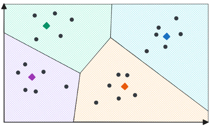
Now, each vector falls within a region. In the context of similarity search, each region consists of vectors that are semantically similar. Since vectors within the same region are more likely to be similar to each other than those in different regions, IVFFlat makes the search process more efficient.
Let’s consider the query vector, as shown in the following image. To find the nearest neighbors to this query vector using IVFFlat, we perform the following steps:
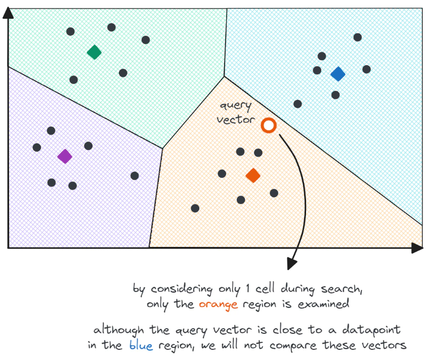
Although the IVFFlat algorithm accelerates the search process and provides good search quality, it can lead to errors. For example, the above image illustrates the scenario where the query vector resides at the edge of two cells. Despite the query vector being close to a datapoint in the blue region, this vector will not be considered a nearest neighbor candidate since the search scope is limited to the orange region.
To address this issue and enhance search quality, we can expand the search scope by selecting several regions to search for nearest neighbor candidates. However, this approach comes with a trade-off: it increases search time.
To create an IVFFlat index using pgvector, two parameters need to be specified:
vector_l2_ops, vector_ip_ops, and vector_cosine_ops, respectively. It is essential to select the same distance metric for both the creation and querying of the index.lists parameter specifies the number of clusters that will be created. Pgvector suggests that an appropriate number of lists is rows/1000 for datasets with up to 1 million rows and sqrt(rows) for larger datasets. It is also advisable to create at least 10 clusters.To create an IVFFlat index in a PostgreSQL table, you can use the following statement:
| |
It is important to note that the index should be created once the table is populated with data.
To search for similar images through the IVFFlat index of the pgvector extension, we can use SQL SELECT statements and the built-in distance operators. The structure of a SELECT statement was explained in the Exact Nearest Neighbor Search blog post. For approximate nearest neighbor search, some additional parameters need to be considered to use the IVFFlat index.
The number of regions to consider during search is determined by the probes parameter. According to pgvector documentation, the recommended value for the probes parameter is sqrt(lists). The default value is 1. To specify the value of the probes parameter, you can execute the following statement:
| |
To specify the number of probes to use for a single query, you should use the LOCAL keyword.
It’s important to note that PostgreSQL does not guarantee the use of an approximate index, as it may determine that a sequential scan could be more efficient for a query. To check whether PostgreSQL utilizes the index in a query, you can prefix the SELECT statement with the EXPLAIN ANALYZE keywords.
| |
An example of a query plan that utilizes the IVFFlat index is provided below:
| |
Additionally, you may need to rewrite (or simplify) your queries in order to use an approximate index. For example, since pgvector only supports ascending-order index scans, the following query does not utilize the IVFFlat index:
| |
If we want to utilize the index, one possible way to rewrite the SELECT statement is as follows:
| |
In the Jupyter Notebook provided on my GitHub repository, you’ll explore text-to-image and image-to-image search scenarios. You will use the same text prompts and reference images as in the Exact Nearest Neighbors search example, allowing for a comparison of the accuracy of the results.

Feel free to experiment with the notebook and modify the code to gain hands-on experience with the pgvector extension!
In this post, you used the IVFFlat indexing algorithm of the pgvector extension to search for paintings that closely match a reference image or a text prompt. In the upcoming post, we will explore the workings of the HNSW index and use it for similarity searches.
If you want to explore pgvector’s features, check out these learning resources:

Explore vector similarity search using the Hierarchical Navigable Small World (HNSW) index of pgvector on Azure Cosmos DB for PostgreSQL.
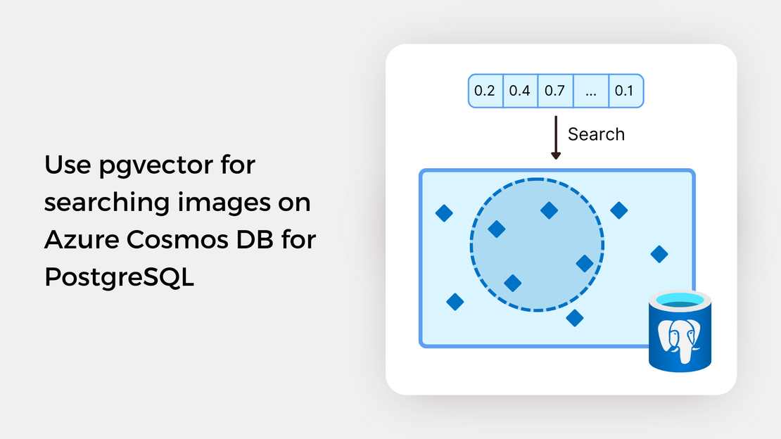
Learn how to write SQL queries to search for and identify images that are semantically similar to a reference image or text prompt using pgvector.

My presentation about vector search with Azure AI Vision and Azure Cosmos DB for PostgreSQL at the Azure Cosmos DB Usergroup.

My presentation about vector search with Azure AI Vision and Azure Cosmos DB for PostgreSQL at the virtual show MVP TechBytes.